from typing import Callable, Tuple,  Union

import pandas as pd
import numpy as np

import jax as jax
import jax.numpy as jnp
import jax.random as jr

import tensorflow as tf
import tensorflow_probability as tfp

import matplotlib.pyplot as plt
import seaborn as sns

sns.set_theme()

jax.config.update("jax_enable_x64", True)In this post, I wanted to walk through the more basic version of the Metropolis-Hastings algorithm. I was asked to implement this algorithm for a coding task at one point and wanted to share my thought process that I went through. So here we go.
The task
Implement a Metropolis Markov chain Monte Carlo algorithm for producing random samples from a normal distribution
\[\begin{equation} f(x)= {\frac{1}{\sigma\sqrt{2\pi}}} e^{- {\frac {1}{2}} (\frac {x-\mu}{\sigma})^2} \end{equation}\]
Tip
The algorithm can target any probability distribution. In this case, we know what it is and that makes things easier but you can change \(f\) to be any probability distribution. That makes them very useful when we have complex models who’s posterior distribution we are trying to target.
Build the model
def make_target_probability_fn(mu, sigma):
    """
    Factory function for the target probability distribution
    """
    def target_probability_fn(x):
        """
        Probability density function for the target distribution
        """
        return jnp.exp(-(x - mu)**2 / (2 * sigma**2)) / (sigma * jnp.sqrt(2 * jnp.pi))
    return target_probability_fn
This could be done by calling in the normal distribution from another library (e.g. scikit-learn or tensorflow_probability) but I wanted to emphasize that this can be any distribution you can code.
# test the function for 1 value:
x = jr.normal(jr.key(1), 1)

print(f'Likelihood: {make_target_probability_fn(0., 1.)(x)}')
Likelihood: [0.19785846]# test the function for multiple values:
x = jr.normal(jr.PRNGKey(1), 10)
print(f'Likelihood: {make_target_probability_fn(0., 1.)(x)}')Likelihood: [0.19785846 0.39625937 0.3930378 0.2522948 0.28200095 0.31425692
0.39780836 0.29784282 0.39843097 0.15984802]Algorithm implementation
Inputs for the algorithm:
- \(N\) number of iterations
- \(\mu\) mean of the normal distribution
- \(\sigma\) standard deviation of the normal distribution
- \(\tau\) step size of Metropolis MCMC
The mean and standard deviation of the normal distribution pertain to the data while the number of iterations and step size are specific to the MCMC algorithm. This provides a natural partition in the architecture of the code. Conveniently, make_target_probability_fn already accounts for the data part of the problem.
To implement the sampling algorithm, we will use a functional programming approach that encodes one-step or iteration of the algorithm. This is known as a state transformer and is analogous to creating the Markov transition kernel for the algorithm. Symbolically, it will look like:
\[\begin{equation} (i, X) \rightarrow ((i+1, X'), z) \end{equation}\] where \(i\) is the iteration, \(X\) is the value, and \(z\) is the change from \(X\) to \(X'\) prime. The internals of the algorithm can be found on Wikipedia.
def make_metropolis_mcmc_one_step(
    tau: jnp.float64,
    target_probability_fn: Callable,
):

    def proposal_fn(state: jnp.float64, key: jr.PRNGKey) -> jnp.float64:
        # X' ~ Uniform(X - tau, X + tau)
        return jr.uniform(key=key, shape=(), minval=state - tau, maxval=state + tau)

    def one_step(carry: Tuple[jnp.float64, jr.PRNGKey], _):
        """
        Performs one step of the Metropolis MCMC algorithm.

        Return a tuple of the state and the key to be carrid along
        """
        # unpack carry
        state, key = carry

        proposal_key, acceptance_key, next_key = jr.split(key, 3)

        # propose new value
        proposed_state = proposal_fn(state, proposal_key)

        # compute acceptance probabiltiy
        acceptance_probability = jnp.minimum(
            1, target_probability_fn(proposed_state) / target_probability_fn(state)
        )

        # accept reject
        next_state = jnp.where(
            jr.uniform(key=acceptance_key, shape=()) < acceptance_probability,
            proposed_state,
            state,
        )

        # carry forward next state and next key
        new_carry = (next_state, next_key)

        return new_carry, next_state

    return one_step
# test function
my_one_step = make_metropolis_mcmc_one_step(
tau=4.4,
target_probability_fn=make_target_probability_fn(mu=0, sigma=1),
)
print(f'Output: {my_one_step((0, jr.PRNGKey(1)), 0)}')Output: ((Array(0., dtype=float64), Array([2441914641, 3819641963], dtype=uint32)), Array(0., dtype=float64))Repeated kernel applications
The last step is to build a function which acts as the “driver” for the sampler to produce the \(N\)-many iterations. We do this using the `jax.lax.scan’ function which performs the following operation:
scan :: (c -> a -> (c, b)) -> c -> [a] -> (c, [b])
The key is that the output is a List structure that contains all of the intermediate states.
def run_mcmc(
    N: int,
    one_step_fn: Callable,
    init_carry: Tuple[jnp.float64, jr.PRNGKey],
):
    """
    Runs the Metropolis MCMC algorithm for a given number of iterations.

    Args:
        N (int): The number of iterations to run the MCMC chain.
        one_step_fn (Callable): A function that performs one step of the
            Metropolis MCMC algorithm.
        init_carry (Tuple[jnp.float64, jr.PRNGKey]): A tuple containing the
            initial state (x0) and the initial JAX PRNGKey.

    Returns:
        Tuple[Tuple[jnp.float64, jr.PRNGKey], jnp.ndarray]: A tuple containing:
            - final_carry (Tuple[jnp.float64, jr.PRNGKey]): The final state and
              PRNGKey after N iterations.
            - states (jnp.ndarray): An array of sampled states from the MCMC chain.
    """
    final_carry, states = jax.lax.scan(one_step_fn, init=init_carry, xs=None, length=N)

    return final_carry, states
Lets now run the MCMC!
init_carry = (10.0, jr.key(1))

_, samples = run_mcmc(N=5000, one_step_fn=my_one_step, init_carry=init_carry)
# plot test run
plt.plot(samples, color = 'navy', alpha = 0.6, label = 'Posterior samples')
plt.hlines(y = jnp.mean(samples), xmin = 0, xmax= 5000, color="orange", label = 'Posterior mean')
txt = f' Acceptance rate: {(1- jnp.mean(samples[1:] == samples[:-1])):.4f}'
plt.title(r'Posterior samples with $\tau$ = 4.4, $x^{(0)}$ = 10' + txt)
plt.show()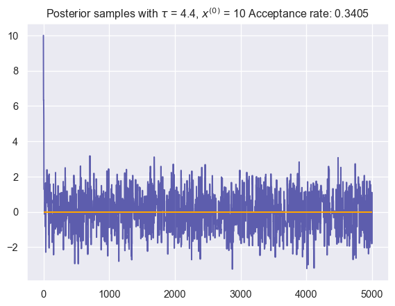
We now have machinery that is highly reusable because of the functional form each takes. We can change any of the functions and the changes will trickle through nicely! It’d be a good exercise to draw a diagram of all of the functions and trace through their interactions.
This blog is part of a bigger series on MCMC and how to code various samplers. Stay tuned for a follow up on an adaptive version of this algorithm that changes the code so we don’t need to worry about manually tuning the sampler.
Thanks for reading
In my spare time, I like to take photos so I’m going to add one photo I like at the end of each post as a thank you :)