# parameter values
beta0 = 1.2
beta1 = 0.5

# random x values
x = np.random.uniform(
    low = 0.0,
    high = 10.0,
    size = 100,
    )
# evaluate mean
mu = beta0 + beta1*x
# simulate y values
y = np.random.normal(
    loc = mu,
    scale = 0.5,
    size = 100
)During my undergraduate degree, I always struggled with the concept of computing statistical quantities. I couldn’t wrap my head around what commands to use in my editor to mimic the math that I could write on the page. Fast forward a several years and lots of coding assignments, I now kind of get it. I’m writing this blog post to highlight one of the nicest links between the math and the computation that I’ve come across and the motivation behind the title of this post - conditional probabilities are partial function applications.
Quick refresher on conditional probabilities
Let’s start with a quick recap of what exactly a conditional probability is. Suppose we have 2 events, \(A\) and \(B\). We say that the conditional probability of B given A is \[P(B \vert A) = \frac{P(A \bigcap B)}{P(A)}\] We assume that \(P(A)>0\). The intuition here is that we are updating our belief about \(B\) knowing that something specific about \(A\) has occured. If these events are independent, then the above equation simplifies since we \(P(A \bigcap B) = P(A) P(B)\) (i.e. knowing something about \(A\) gives you no additional information about \(B\)).
However, conditional probability extends far beyond simple events. In statistical modeling, conditional probabilities form the backbone of likelihood-based inference. When we model data, we often use conditional probabilities to express how likely the observed data is, given a set of model parameters (data generating model). This is where the likelihood function comes into play. The likelihood function is an unnormalized probability distribution that is a function of the model parameters, not the data. It captures the plausibility of the parameters given the data, and by conditioning on different parameters, we can explore various hypotheses or refine our model.
For example, in Bayesian inference, we condition on observed data to update our prior beliefs about the model parameters, yielding the posterior distribution. This conditional framework underpins nearly all of modern statistical inference, from maximum likelihood estimation to more complex Markov Chain Monte Carlo inference schemes. These likelihood functions can be very easy to write on paper but difficult to code and that’s what I want to dive into here. Let’s define a model with two parameters. \[y_i \sim N(\beta_0 + \beta_1 x_i, 2^2)\] Some may recognize this as a linear regression. Our dependent random varialbe \(y\) follows a Normal distribution which has a mean that depends on a linear transformation of the independent variable \(x\). We can write out the likelihood function of this model using the probability density function of the Normal. \[\begin{align} L(\beta_0, \beta_1 ; x) &= \prod_{i = 1}^n P(y_i) \\ &= \prod_{i = 1}^n \frac{1}{\sqrt{2 \pi \cdot0.52^2}} e^{-\frac{(y_i - (\beta_0 + \beta_1 x_i))^2}{2 \cdot 0.5^2}} \end{align}\] Here’s a simulated data set from this model.
# Scatter plot of the data
plt.scatter(x, y, label="Data points", color='blue')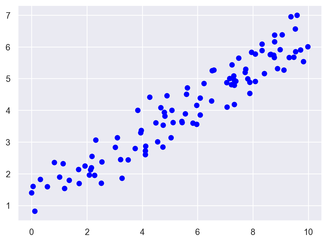
Partial function applications
In Python, partial function applications is a feature provided by functools package with the partial function. It allows you to take a function and fix some of its arguments, returning a new function that takes fewer arguments. The similarity to conditional probabilities lies in this idea of fixing known inputs. This is a nice feature of Python - we can pass around functions as first class objects (an entity that can be dynamically created, destroyed, passed to a function, returned as a value, and have all the rights as other variables in the programming language have).
Let’s look at an example.
from functools import partial def my_function(a, b):
"""
A function that takes two arguements and returns the product
"""
return a*bWe can partially apply the function by “fixing” one of the parameters values to a specific value. For example, fix a=2.
multiply_by_2 = partial(my_function, a = 2)

print(multiply_by_2)                        # this returns a function
print(multiply_by_2(b = 4))                 # this returns 8
functools.partial(<function my_function at 0x14f4972e0>, a=2)
8Here we used partial to create a new function that fixes one of the arguments to 2, hence the new function is multiplies the input by 2. If the arguments to the my_function correspond to parameter values in my model and the output is the likelihood function, then applying partial returns the conditional likelihood.
Why does this analogy work?
The analogy between partial function applications and conditional probability is very nice because both involve reducing complexity by “conditioning” on known information. In statistics, we’re conditioning on known events/realizations, while in programming, we’re fixing known inputs/data.
Consider this: when you fix one argument of a function, you’re effectively “conditioning” the function on that known value. Similarly, conditional probability refines the likelihood of an event by fixing certain known information. This way of thinking can be particularly powerful when designing simulations or modeling problems where we frequently update our beliefs based on new information.
Apply it to our model
Lets create the likelihood function of our model. I’m going to take advantage of the logpdf method of the normal distribution which ‘scipy’ has already implemented. It’s always good practice to allocate these computations to well tested and documented libraries so we avoid any algebraic mistakes in our code.
def model_likelihood(beta0, beta1):
    log_probs = sp.stats.norm(
        loc = mu,           # model mean - computed as global variable earlier
        scale = 0.5         # fixed variance
        ).logpdf(y)         # log prob of observed random variables
    return np.sum(log_probs)

# test arbitrary values
print(f"log-prob eval: {model_likelihood(beta0 = 0.1, beta1 = 0.1)}")
log-prob eval: -72.04687255986312Now we can use the partial to get the conditional likelihood of beta0 given beta1.
conditional_likelihood = partial(model_likelihood, beta1 = 0.1)

print(f"Conditional log-likelihood: {conditional_likelihood}")
print(f"Check: {conditional_likelihood(beta0= 0.1)}")
Conditional log-likelihood: functools.partial(<function model_likelihood at 0x14f4971a0>, beta1=0.1)
Check: -72.04687255986312And they are the same as before! This mirrors how we compute conditional probabilities by progressively refining our estimate as more information becomes available. For example, if you found some information saying that beta1 should be 0.5, you can fix that using this technique. All you need to do then is optimize the (log) likelihood for the other parameter.
Closing thoughts
The parallel between partial function applications and conditional probabilities provides an intuitive bridge between coding and probability theory. By conditioning on known values, both in probability and programming, we can simplify complex systems and gain clearer insights into the behavior of the remaining uncertainties.
In your next coding or probability problem, try thinking of how partial applications might represent conditioned states of knowledge. This perspective can make otherwise complex ideas feel a bit more manageable—and highlight the deep connections between computation and probability theory.
Thanks for reading
In my spare time, I like to take photos so I’m going to add one photo I like at the end of each post as a thank you :)