flowchart LR
  A(Susceptible) --> B(Infected)
When I started my PhD two years ago, I had never looked at an epidemic model outside of an elementry differential equations course. Fast forward two years, and one Covid-19 later, the bulk of my work is centred around epidemic models. More specifically, stochastic epidemic models. Differential equation models are simple and easy to use but are often too rigid since they don’t reflect the randomness we see in the real world when it comes to the spread of disease.
This post is going to be a tutorial that I wish I had at the start of my epidemic modelling journey. The aim is to implement/code a chain binomial epidemic model in Python. This model is sometimes referred to as the Reed-Frost model and was initially used to model epidemic spread in the late 1920s (more details1). It is one of the simplest epidemic models as it only focuses on the infection process so take this as the base case. Future posts will dive deeper into the mathematics and how to expand on this model to make it more realistic.
Reed-Frost model
The Reed-Frost model helps us predict the number of people who will become infected over time, given some initial conditions.
Intuition
Imagine a group of people where some are initially infected with a disease, and others are susceptible but not yet infected. The Reed-Frost model works by dividing time into discrete steps2, such as days or weeks. At each time step, each susceptible person has a chance of getting infected based on their contact with infectious individuals.
At the beginning of the outbreak, the population is divided into two groups: susceptible (those who can get infected) and infectious (those who are currently infected). If we were to think of this as a graphical representation, it would be a 2 compartment model.
Now the question becomes how do individuals move between these states. The model uses a probability parameter to represent the likelihood that a susceptible person will get infected upon contact with an infectious person. This probability is often denoted as \(p\).
The process unfolds over a series of discrete time steps. At each step, every susceptible individual has a chance to become infected if they come into contact with any infectious individuals (this is a very loose way to apply some mathematical structure to a very complex infection transmission mechanism).
The number of new infections at each time step depends on the number of susceptible and infectious individuals and the probability of transmission. The model assumes that once a person is infected, they remain infectious for only one time step.
Why this is a good starting
The Reed-Frost model is powerful because it captures the essential dynamics of disease transmission in a straightforward manner. It considers the key factors that drive an epidemic: the number of susceptible individuals, the number of infectious individuals, and the probability of transmission. By iterating this process over multiple time steps, the model can simulate the spread of an infection and help predict its potential impact on the population.
Python implementation
For this tutorial, I am going to try to use as few packages as possible so I’m going to restrict myself to only numpy and pandas. The rest of the code will be base Python.
# load packages
import numpy as np
import pandas as pd

import matplotlib.pyplot as plt
import seaborn as sns

sns.set()
Let’s take stock of what we know at this point. The Reed-Frost model which is a 2-state compartmental model.
Important
This is a class of models and not a specific model.
To specify a model we need to add more structure. We want to know the size of population the disease is spreading through, the duration of each step in which events are happening (recall this is a discrete time model), and the last is going to be the transition rate or epidemic dynamics (how the disease is transmitted). The assumptions are as follows:
- 100 epidemic units3 with 99 susceptibles and 1 infected units. This is represented as a vector \([S_0, I_0] = [99,1]\) (the subscript \(i\) is the time period).
- Time period is going to be daily so we set the time delta \(\triangle d = 1\).
- Epidemic dynamics will be a density based transmission where we ‘count’ the number of pairwise interactions between infectious units and susceptibles and divide by the population size. This means that the probabilty of an infection happening has a rate of \(\lambda_i= \beta \frac{S_i I_i}{S_i + I_i}\) which translates into a probability of \(p_i = \exp\{- \lambda_i * \triangle d \}\)4.
# initial values
time_delta = 1.                 # 1 day
initial_pop = [99.,1.]          # population vector
parameters0 = 0.01              # daily transmission parameter
With the constants and initial conditions set, its time to move to the main bit of the code which performs the simulation.
Tip
I’ve been using the term implementing a model and this doesn’t really have a set definition. In this case, implementation is done when you can simulate a correct trajectory of the epidemic but in other settings it may mean fitting a model to data, validating, predicting, etc. The scope of an implementation changes with the nature of the problem and is context specific. Its all jargon here.
The function below called SI_iteration takes 3 parameter values: 1. parameters - this is a vector of model parameters. For now, this is a 1D vector holding the value for \(\beta\). 2. state - this is a 2D vector containing the counts for each of the states. 3. time_delta - the size (in days) of the discrete time step
def SI_iteration(parameters, state, time_delta):
beta = parameters
num_susceptibles, num_infected = state
# Step 1: compute transition rates
SI_rate = beta*(num_susceptibles * num_infected)/(num_susceptibles + num_infected)
# Step 2: convert event rates to probabilities
i_rate = 1 - np.exp(- SI_rate * time_delta)
# Step 3: simulate number of new infections
num_new_infections = np.random.binomial(num_susceptibles, i_rate)
# Step 4; state update
return [num_susceptibles - num_new_infections, num_infected + num_new_infections]- 1
- Compute the transition rate
- 2
- Turn the transition rate into a probability of new infections
- 3
- Sample the number of new infections
I’m going to ignore the mathematics of Step 2 in chunk above for now since that will be its own post down the line. The gory details can be found in the paper I mentioned earlier for those curious. Now for using our new function! Taking the initial values for each of the arguments and plugging them in, we can get the outcome of a single iteration or single step of our epidemic process. This is not a complete path!
# single iteration/forward step
np.random.seed(20240701)
new_state = SI_iteration(parameters0, initial_pop, time_delta)
print(f'New state: {new_state}')- 1
- Set the seed for reproducible value.
New state: [98.0, 2.0]Simulate a path
We can extend the single iteration to sample a full path of the epidemic by calling our function over and over again. This is not the most efficient way of performing a simulation but it is easy to understand so it’ll do for now.
# simulate full path
def simulate(initial_state, num_steps):
    # counters
    ii = 0
    S = np.zeros(num_steps)
    I = np.zeros(num_steps)

    # unpack the state
    S[0], I[0] = initial_state
    state = initial_state

    while ii < num_steps:
      # single iteration to update the state
      state = SI_iteration(parameters0, state, time_delta)
      # record the outcome
      S[ii], I[ii] = state

      ii += 1

    return {'Time': np.cumsum(np.repeat(time_delta, num_steps)),
            'Susceptible': S,
            'Infected': I}
And run a simulation of 100 steps (note that some of the steps might be non-events since every unit has progressed through the epidemic). There are nice ways of stopping simulations early by using a clever stop condition within the while loop.
sample_epi = simulate(initial_pop, 100)

pd.DataFrame(sample_epi).head(10)| Time | Susceptible | Infected | |
|---|---|---|---|
| 0 | 1.0 | 99.0 | 1.0 |
| 1 | 2.0 | 97.0 | 3.0 |
| 2 | 3.0 | 94.0 | 6.0 |
| 3 | 4.0 | 86.0 | 14.0 |
| 4 | 5.0 | 74.0 | 26.0 |
| 5 | 6.0 | 56.0 | 44.0 |
| 6 | 7.0 | 41.0 | 59.0 |
| 7 | 8.0 | 35.0 | 65.0 |
| 8 | 9.0 | 29.0 | 71.0 |
| 9 | 10.0 | 21.0 | 79.0 |
Lets plot the simulation!
plt.figure(figsize=(12, 7))

S_line = plt.plot("Time","Susceptible", data=sample_epi, color="b", linewidth=2)
I_line = plt.plot("Time","Infected", data=sample_epi, color="r", linewidth=2)

plt.xlabel("Days",fontweight="bold")
plt.ylabel("Count",fontweight="bold")

legend = plt.legend(title="Population",loc=5,bbox_to_anchor=(1.2,0.5))
frame = legend.get_frame()
frame.set_facecolor("white")
frame.set_linewidth(0)

# Add labels and title
plt.xlabel('Days', fontweight="bold")  # Add x-axis label with font styling
plt.ylabel('Count', fontweight="bold")  # Add y-axis label with font styling
plt.title('Single path simulation', fontsize=16)  # Add plot title with font size

plt.show()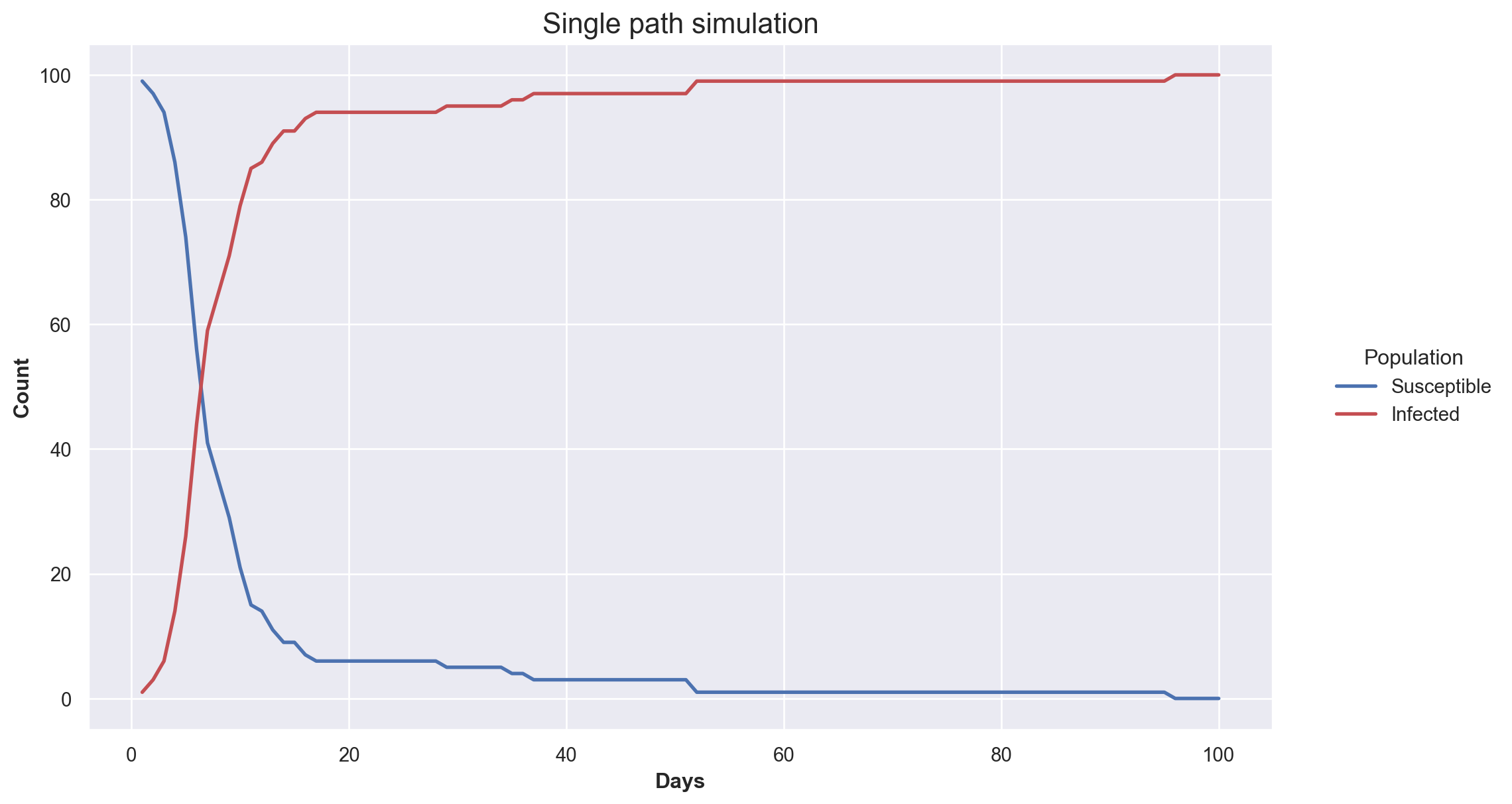
Conclusion
In this tutorial, I showed one way to implement a chain binomial epidemic model. This basic model is a great starting point for building more complex and realistic models. The function SI_iteration uses a simplified version of the Gillespie algorithm which is the standard algorithm for simulating stochastic trajectories for these types of systems. I’d also recommend checking out this blog post by Lewis Cole for an in depth look at the algorithm.
Next steps
As far as using epidemic models in the real world goes, simulation is only one half of the coin. The other side has to do with fitting these models. If the problem was reversed and we had observed an epidemic process, recorded the data and created a data set that looks something like @epi_dataset we could then try to find the value of parameters which generated that data. This can be done in a variety of ways such as maximum likelihood estimation or Bayesian inference. If this type of problem interests you, I’d highly recommend checking out the IDDinf 2024 inference course. This is a course I will be co-teaching with some incredible people in September 2024 and will go over everything you need to know to fit epidemic models with Bayesian inference.
Thanks for reading
In my spare time, I like to take photos so I’m going to add one photo I like at the end of each post as a thank you :) 
Footnotes
I usually work with continuous time models which pose their own challenges. More on this will come in later posts↩︎
An epidemic unit can be anything that we can classify as susceptible or infected. These models are used for humans and animals so its easier to generalize the concept of an epidemic unit. The units can even be aggregated to represent households or farms. It gives us a more flexibility to adapt the scope of the model.↩︎
Future post on the interpretable mathematics of epidemic models↩︎